 Building an effective air pollution control plan requires information of the contribution of various sources. This is not an easy or a quick process, as it involves many steps from field experiments, to laboratory analysis, to (statistical and predictive) modeling, and some related to linking the results to pollution control plans. We structured a primer on the steps of source apportionment, explaining the process using 2 approaches to support an informed air quality management plan. You can download a pdf version of the primer here or browse the individual pages below.
First edition of this primer from 2011 is available here.
Some background notes on pollution source apportionment is explained in the following tables.
- What is particulate matter (frequently asked questions)
- Pros and cons of top-down (receptor-based) and bottom-up (emissions-based) methods
- Information and decisions required to conduct top-down (receptor-based) source apportionment
- Laboratory techniques for chemical analysis of filter samples
- Elemental markers for various sources detected during chemical analysis
- Comparison of model requirements, strengths, and limitations of receptor models
 |
 |
 |
 |
 |
 |
 |
 |
 |
 |
 |
 |
 |
 |
 |
 |
 |
 |
 |
 |
 |
 |
 |
 |
- Tools for improving air quality management: A review of top-down source apportionment techniques and their application in developing countries. Publication by the World Bank (2011) [Click here for a PDF]
- An 101 overview of “air pollution monitoring“
- A version of the pros-cons table was published in Accelerating city progress on clean air: Innovation and action guide – Technical report with Vital Strategies (New York, USA, 2020) Download
Pros and Cons of Source Apportionment Methods
| Category | Bottom-up source modelling approach | Top-down receptor modelling approach |
|---|---|---|
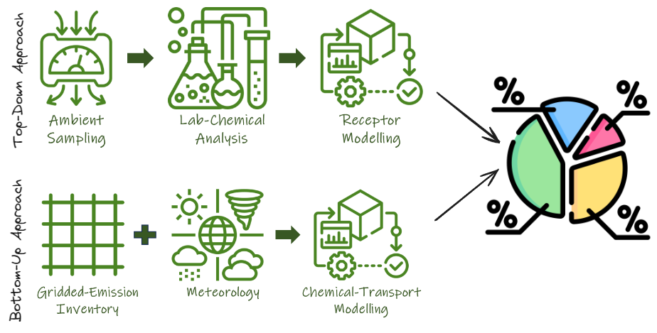
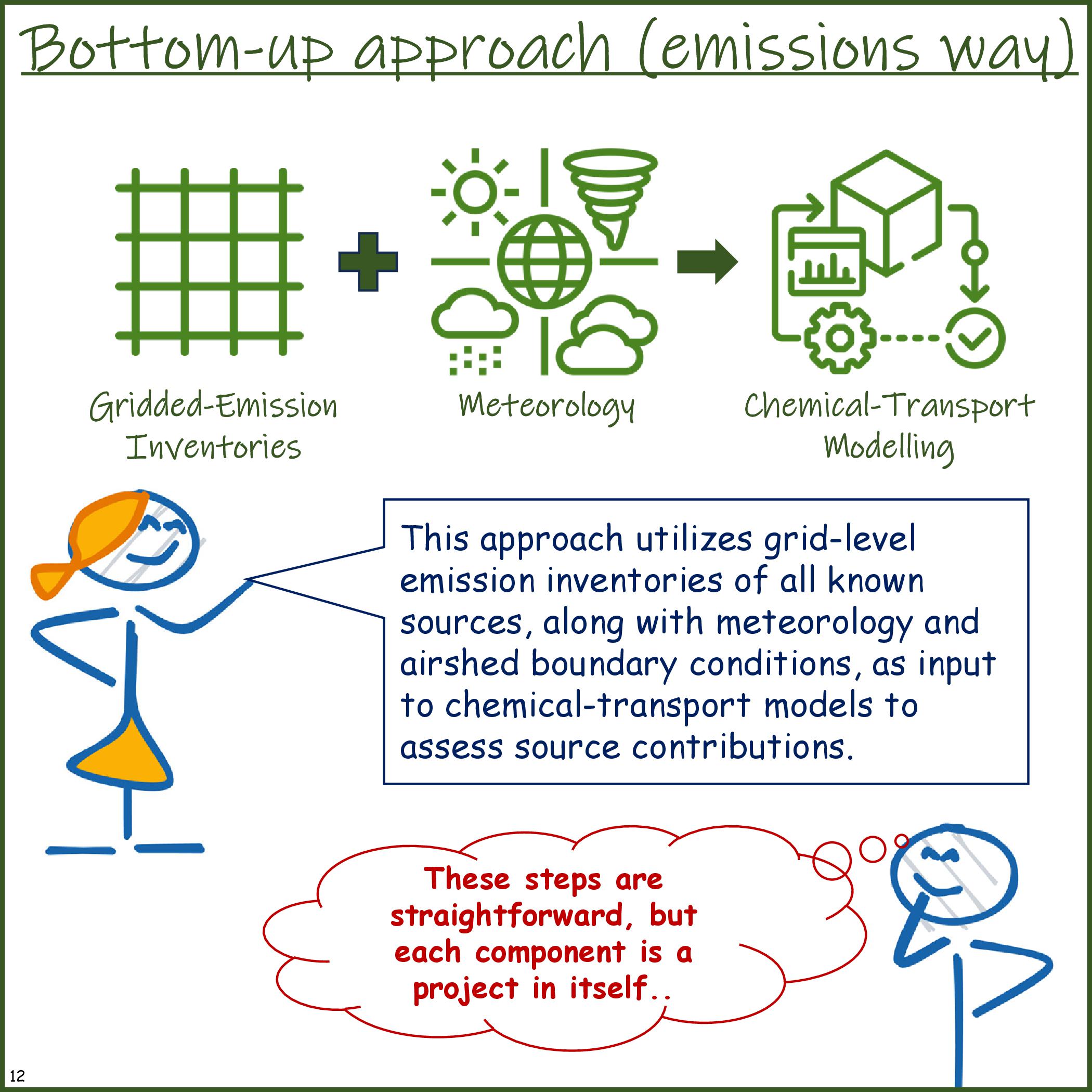
| basic definition | In this approach an emissions inventory is established for all the known sectors (anthropogenic and natural) and processed through a meteorology coupled chemical transport model to ascertain their share of contribution to the select airshed. | In this approach, an ambient sample is analysed for its chemical composition (in the form of ions, metals, and carbon species) and statistically matched with the chemical profiles of different fuels to ascertain their share of contribution to the measured ambient sample. |
| source definition | Typically, source refers to a sector and in some cases, it can refer to a region. | Typically, source refers to the type of fuel and with some handwaving it can refer to a sector. |
| Major limitations | The emissions inventory work is heavily dependent on the depth of activity levels, fuel consumption data, and emission factors which vary by region and combustion technology in place. | It is very difficult to differentiative between the sectors burning the same fuels. For example, diesel burnt at a generator set and diesel burnt in a truck will show the same chemical profile; dust from wind erosion and dust from the side of the roads that is resuspended will have the same chemical profile; biomass burnt in an open field and biomass burnt inside the house for cooking will have the same chemical profile. |
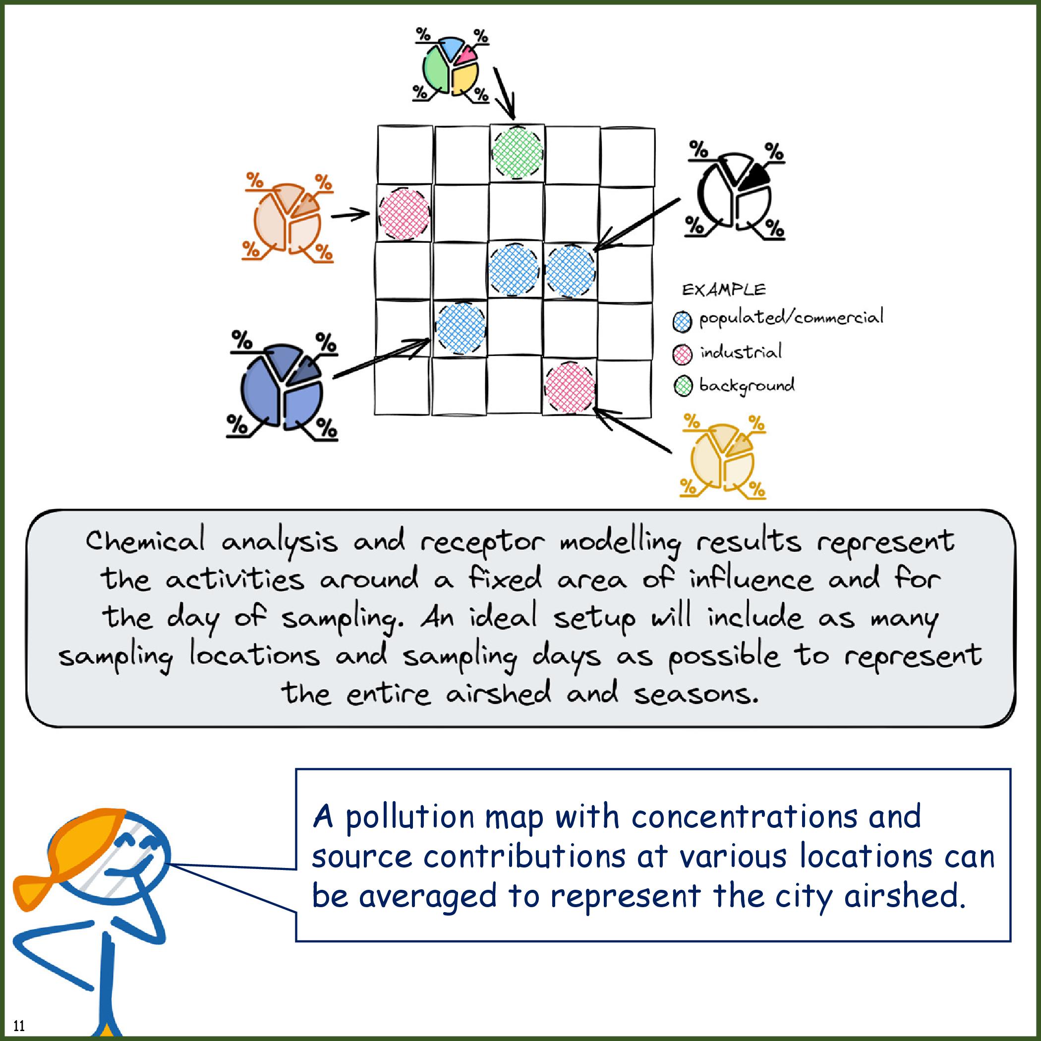
| Spatial representativeness | Analysis results are representative of the entire airshed selected for the emissions and the chemical transport modelling exercise. The grid resolution can provide further details within the airshed. | Analysis results are representative of an area covering 2-km radius of the sampling location. The representativeness of the overall result to a city or a region depends on the number of sampling locations and the number of samples collected in the city or the region. |
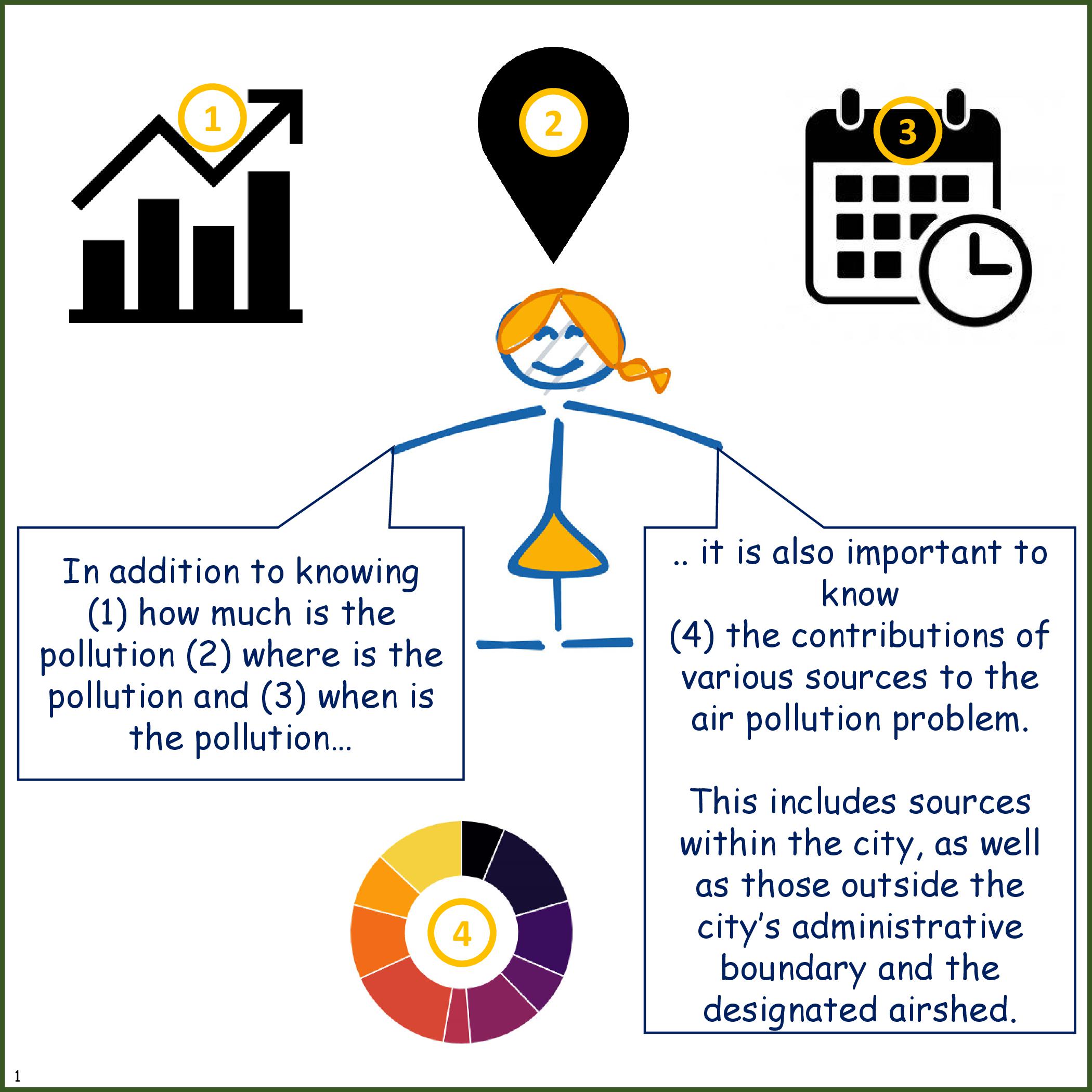
| Temporal representativeness | Analysis results will be available at various temporal scales by hour, by day, by month, and by season, depending on the granularity of the emissions and the chemical transport modelling exercise. | Analysis results are representative of the day and time of the sample collected. Because of this, multiple samples are required by month and season to ascertain the temporal trends in source contributions. |
| Financial burden | VARIABLE - depending on the granularity of the emissions and chemical transport modelling exercise; primary data collecting activities; and modelling tools employed. | HIGH - depending on the number of sampling locations in the airshed and number of samples collected per season. |
| Laboratory needs | HIGH - when primary data collection is carried out to ascertain the emission factors by fuel and by sector. | HIGH - a stringent set of protocols must be followed starting from sampling, storage, chemical analysis, source profiling, QAQC, and receptor modelling. |
| Personnel needs | LOW to MEDIUM - when the emission inventories are available and the chemical transport model setup is operational, personnel needs can be low. | HIGH - Includes personnel to perform field, laboratory and statistical modeling tasks as described below. Advanced, semi-autonomous samplers can reduce personnel time in the field. |
| Personnel skill needs | HIGH - experienced staff is required to collate/manage/map/analyse the emissions inventory for the airshed; experienced staff is required to operate/calibrate/analyse the meteorology coupled chemical transport models for the airshed to ascertain the source contributions | HIGH - experienced staff is required to collect/store/record the samples during the field experiment; experienced staff is required to operate/calibrate/analyse the samples in the lab; and experienced staff is required to conduct the receptor modelling exercise involving selection and use of relevant source profiles. |
| Computational needs | HIGH - depending on the chemical transport model of choice, chemical mechanism selected, spatial and temporal resolution of the modelling system, and range of output parameters, computational needs can range from HIGH to VERY HIGH | MINIMUM - only part when computational facilities are required is the receptor modelling exercise, which is a statistical package capable of running on a laptop |
| Study time scales | Typically, less than one year. | Typically, one year for the sample exercises and 1-2 years for chemical analysis and receptor modelling (which entirely depends on the capacity of the lab) |
Laboratory Techniques for Chemical Analysis
| Measurement | Suitable Analytical Technique |
|---|---|
| Particle mass | Gravimetric analysis, b-gauge monitoring |
| Elements (Na, Mg, Al, Si, P, S, Cl, K, Ca, Ti, V, Cr, Mn, Fe, Co, Ni, Cu, Zn, Ga, As, Se, Br, Rb, Sr, Y, Zr, Mo, Pd, Ag, Cd, In, Sn, Sb, Ba, La, Au, Hg, Ti, Pb and U) | X-Ray Fluorescence, Proton Induced X-ray Emission, Instrumental Neutron Activated Analysis, Inductively Coupled Plasma Spectroscopy, Emission Spectroscopy, Atomic Absorption Spectrophotometry |
| Ions (F-, Cl-, NO2-, PO43-, Br-, SO42-, NO3-, K+, NH4+, and Na+) | Ion Chromatography |
| Ions (Cl-, NO2-, SO42-, NO3- and NH4+) | Automated Colorimetric Analysis |
| Total Carbon | Thermal Combustion Method |
| Individual organic compounds | Solvent Extraction Method followed by Gas Chromatography - Mass Spectroscopy |
| Total Carbon, Elemental Carbon, Organic Carbon, Carbonate Carbon | Thermal Manganese Oxidation Method,Thermal Optical resistance or Thermal/Optical Transmission Method |
| Absorbance (light absorbing carbon) | Optical Absorption, Transmission Densitometry, Integrating Plate or Integrating Sphere Method |
Elemental Markers Detected in Emissions Sources
| Emission Source | Marker Elements (in the order of priority) |
|---|---|
| Soil | Al, Si, Sc, Ti, Fe, Sm, Ca |
| Road dust | Ca, Al, Sc, Si, Ti, Fe, Sm |
| Sea salt | Na, Cl, Br, I, Mg |
| Oil burning | V, Ni, Mn, Fe, Cr, As, S, SO4 |
| Coal burning | Al, Sc, Se, Co, As, Ti, Th, S |
| Iron and steel industries | Mn, Cr, Fe, Zn, W, Rb |
| Non- Ferrous metal industries | Zn, Cu, As, Sb, Pb, Al |
| Glass industry | Sb, As, Pb |
| Cement industry | Ca |
| Refuse incineration | K, Zn, Pb, Sb |
| Biomass burning | K, EC, OC, Br |
| Automobile gasoline | EC, Br, Ce, La, Pt, SO4, NO3 |
| Automobile diesel | OC, EC, S, SO4, NO3 |
| Secondary aerosols | SO4, NO3, NH4 |
Information and Decisions Necessary for Receptor-based Methods
| Steps | Description |
|---|---|
| Background | Specific information on spatial and temporal trends in pollution, types of sources inside and outside the city, potential hot spots (industrial, transport, and residential), physical characteristics of the city, criteria pollutants of interest, and local capacity to conduct source apportionment. |
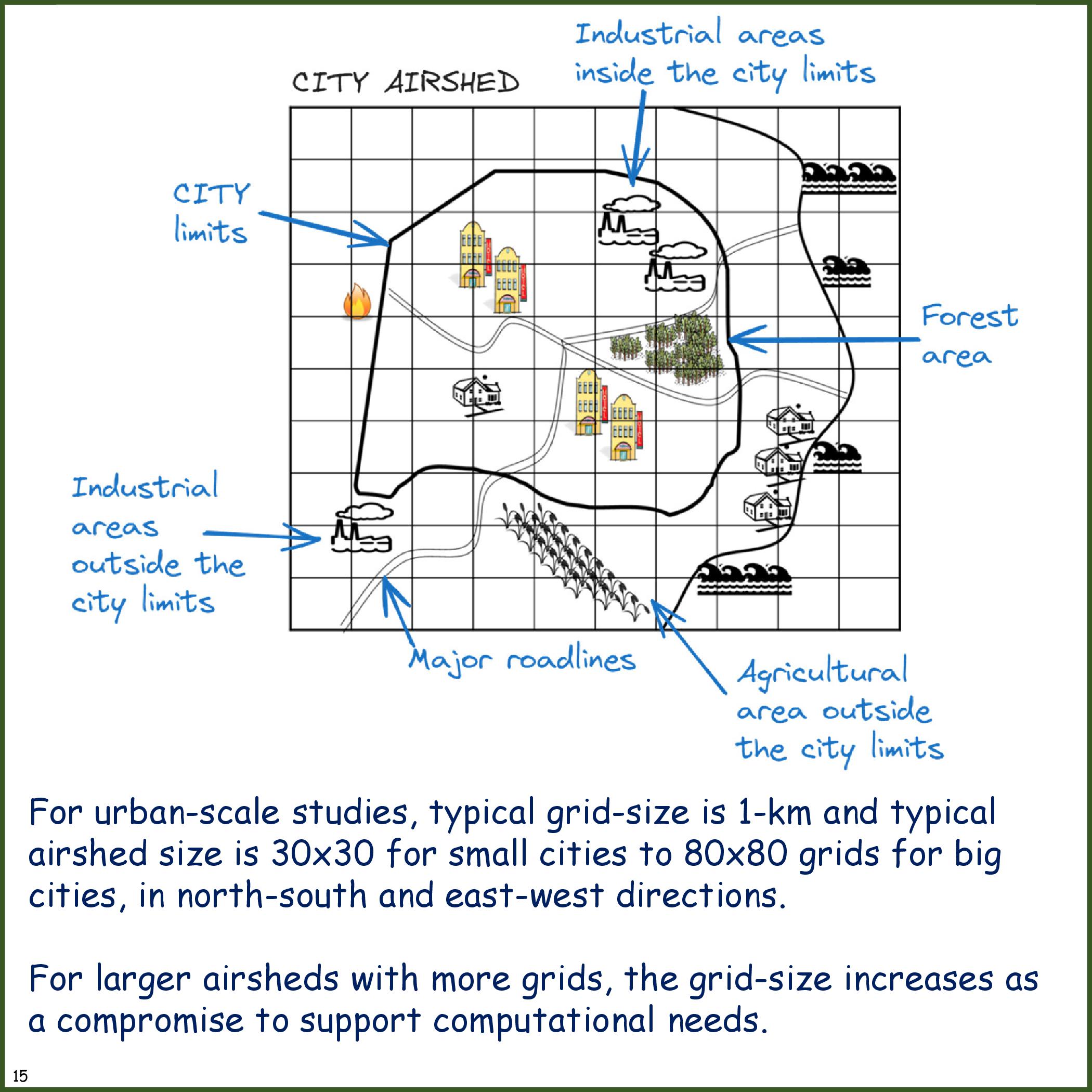
| Site Location | Numbers of sites and decisions on locations with good representativeness of city sources and pollutant mix. Ideally for an airshed of 40km x 40km, at least 15 sites are required to spatially and temporally represent pollution trends. Anything less is a decision dependent financial and operational capacity. |
| Sampling Frequency | Frequency of sampling is partly determined by the study objectives. For example, continuous samplers used for compliance will be operating every day, while others may operate only on a seasonal basis. This decision also depends on the type of sampler available. Ideally, sampling must be conducted for at least 15 days at every site in every representative season. |
| Samplers | Type of sampler and filter media is based on the availability of compatible chemical analysis techniques |
| Chemical Analysis | Level of analysis intended is dependent on the availability of instruments and capacity to operate. See the list of techniques possible. |
| Receptor Modeling | Selection of a receptor model is dependent on the level of chemical analysis conducted in the study. See the table on pros and cons of receptor models. |
| Emission Inventory | While emission inventories are not directly utilized in a top-down analysis, they are useful in estimation of source strengths and identification of source profiles to help ensure efficient and effective receptor modeling is conducted. For example, having an emission inventory can assist in determining where to locate receptors including determining the location of possible hot spots. |
| Source Profiles | Local specific source profiles are desired, but availability of profiles from representative regions may be acceptable. |
| Decision Making | Based on the apportionment results, review of possible technical, institutional, economic, and policy measures. |
Strengths and Limitations of Receptor Models
| Receptor Model | Model Requirements | Strengths | Limitations |
|---|---|---|---|
| Chemical Mass Balance (CMB) | (a) Source and receptor measurements of stable aerosol properties that can distinguish source types. (b Source profiles (mass abundances of physical and chemical properties) that represent emissions pertinent to the study location and time. (c) Uncertainties that reflect measurement error in ambient concentrations and profile variability in source emissions. (d) Sampling periods and locations that represent the effect (e.g., high PM, poor visibility) and different spatial scales (e.g., source dominated, local, regional). | (a) Simple to use, software available. (b) Quantifies major primary source contributions with element, ion, and carbon measurements. (c) Quantifies contributions from source sub-types with single particle and organic compound measurements. (d) Provides quantitative uncertainties on source contribution estimates based on input data uncertainties and colinearity of source profiles. (e) Has potential to quantify secondary sulfate contributions from single sources with gas and particle profiles when profiles can be “aged” by chemical transformation models. | (a) Completely compatible source and receptor measurements are not commonly available. (b) Assumes all observed mass is due to the sources selected in advance, which involves some subjectivity. (c) ~ Does not directly identify the presence of new or unknown sources. (d) Typically does not apportion secondary particle constituents to sources. Must be combined with profile aging model to estimate secondary PM. (e) Much co-linearity among source contributions without more specific markers than elements, ions, and carbon. |
| Injected Marker CMB Tracer Solution | (a) Non-reactive marker(s) added to a single source or set of sources in a well-characterized quantity in relative to other emissions. Sulfur hexafluoride, perfluorocarbons, and rare earth elements have been used. | (a) Simple, no software needed. (b) Definitively identifies presence or absence of material from release source(s). (c) Quantifies primary emissions contributions from release source(s). | (a) Highly sensitive to ratio of marker to PM in source profile; this ratio can have high uncertainty. (b) Marker does not change with secondary aerosol formation—needs profile aging model to fully account for mass due to “spiked” source. (c) Apportions only sources with injected marker. (d) Costly and logistically challenging. |
| Enrichment factor (EF) | (a) Inorganic or organic components or elemental ratios in a reference source (e.g., fugitive dust, sea salt, primary carbon). (b) Ambient measurements of same species. | (a) Simple, no software needed. (b) Indicates presence or absence of emitters. (c) Inexpensive. (d) Provides evidence of secondary PM formation and changes in source profiles between source and receptor. | (a) Semi-quantitative. More useful for source/process identification than for quantification. |
| Multi Linear Regression (MLR) | (a) 100 or more samples with marker species measurements at a receptor. (b) Minimal covariation among marker species due to common dispersion and transport. | (a) Operates without source profiles. (b) Abundance of marker species in source is determined by inverse of regression coefficient. (c) Apportions secondary PM to primary emitters when primary markers are independent variables and secondary component (e.g. SO4=) is dependent variable (d) Implemented by many statistical software packages. | (a) Marker species must be from only the sources or source types examined. (b) Abundance of marker species in emissions is assumed constant with no variability. (c) Limited to sources or source areas with markers. (d) Requires a large number of measurements. |
| Eigen Vector Analysis - Includes Principal Component Analysis (PCA), Empirical Orthogonal Functions (EOF), Postive Matrix Factorization (PMF), and UNMIX | (a) 50 to 100 samples in space or time with source marker species measurements. (b) Knowledge of which species relate to which sources or source types. (c) Minimal co-variation among marker species due to common dispersion and transport. (d) Some samples with and without contributing sources. | (a) Intends to derive source profiles from ambient measurements and as they would appear at the receptor. (b) Intends to relate secondary components to source via correlations with primary emissions in profiles. (c) Sensitive to the influence of unknown and/or minor sources. | (a) Most are based on statistical associations rather than a derivation from physical and chemical principles. (b) Many subjective rather than objective decisions and interpretations. (c) Vectors or components are usually related to broad source types as opposed to specific categories or sources. |
| Time Series | Sequential measurements of one or more chemical markers. 100s to 1000s of individual measurements. | (a) Shows spikes related to nearby source contributions. (b) Can be associated with highly variable wind directions. (c) Depending on sample duration, shows diurnal, day-to day, seasonal, and inter-annual changes in the presence of a source. | (a) Does not quantify source contributions. (b) Requires continuous monitors. Filter methods are impractical. |
| Aerosol Evolution - Includes Box, Guassian, and Eulerian chemical transport modeling | (a) Emissions locations and rates. (b) Meteorological transport times and directions. (c) Meteorological conditions (e.g., wet, dry) along transport pathways. | (a) Can be used parametrically to generate several profiles for typical transport/ meteorological situations that can be used in a CMB. | (a) Very data intensive. Input measurements are often unavailable. (b) Derives relative, rather than absolute, concentrations. (c) Level of complexity may not adequately represent profile transformations. |
| Aerosol Equilibrium | (a) Total (gas plus particle) SO4=, NO3-, NH4+ and possibly other alkaline or acidic species over periods with low temperature and relative humidity variability. (b) Temperature and relative humidity. | (a) Estimates partitioning between gas and particle phases for NH3, HNO3, and NH4NO3. (b) Allows evaluation of effects of precursor gas reductions on ammonium nitrate levels. | (a) Highly sensitive to T and RH. Short duration samples are not usually available. (b) Gas-phase equilibrium depends on particle size, which is not usually known in great detail. (c) Sensitivity to aerosol mixing state not understood/quantified. |