Summary of PM2.5 Pollution and Meteorology Forecast for Today at the state-level (more resources here)

Asansol is the second largest city in the state of West Bengal after the state capital, Kolkata. Asansol is geographically part of the Chota Nagpur plateau and lies on the banks of the Damodar river. The Damodar valley is a major coal mining area (the cities of Durgapur and Dhanbad rely on coal industry and are part of the same valley). The economy is thus driven by the steel and coal sector. The IISCO (Indian Iron and Steel Company Ltd) steel-making plant at Kulti was the first such facility in India. In 2006, it merged with the Steel Authority of India Ltd (SAIL). The plant’s capacity is now 2.5 MT of saleable steel, using what will be the biggest blast furnace in the country.
![]() Eastern Coalfields, which has its headquarters in Sanctoria near Dishergarh, has a significant presence in the area due to the huge deposits of high-quality coal. However, most of the coalfields and surrounding residential colonies are located away from the main city. Nearby areas like Ranigunj, Chinakuri, and Jamuria are of particular importance as coal blocks. As of 2012, the total coal reserve in the ECL command area up to 600 metre depth was 49.17 billion tonnes. Asansol, with a population of 1.15 million (2011 census) over an area of 325 square kilometers, is administered by the Asansol Municipal Corporation.
Eastern Coalfields, which has its headquarters in Sanctoria near Dishergarh, has a significant presence in the area due to the huge deposits of high-quality coal. However, most of the coalfields and surrounding residential colonies are located away from the main city. Nearby areas like Ranigunj, Chinakuri, and Jamuria are of particular importance as coal blocks. As of 2012, the total coal reserve in the ECL command area up to 600 metre depth was 49.17 billion tonnes. Asansol, with a population of 1.15 million (2011 census) over an area of 325 square kilometers, is administered by the Asansol Municipal Corporation.
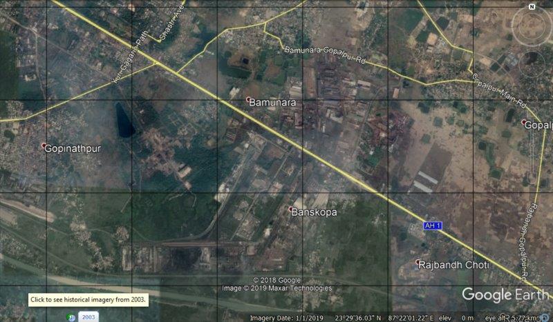
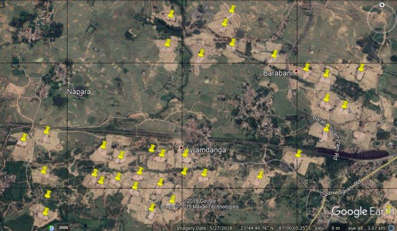
To assess Asansol’s air quality, we selected an airshed covering 60km x 40km. This domain is further segregated into 1km grids, to study the spatial variations in the emission and the pollution loads.
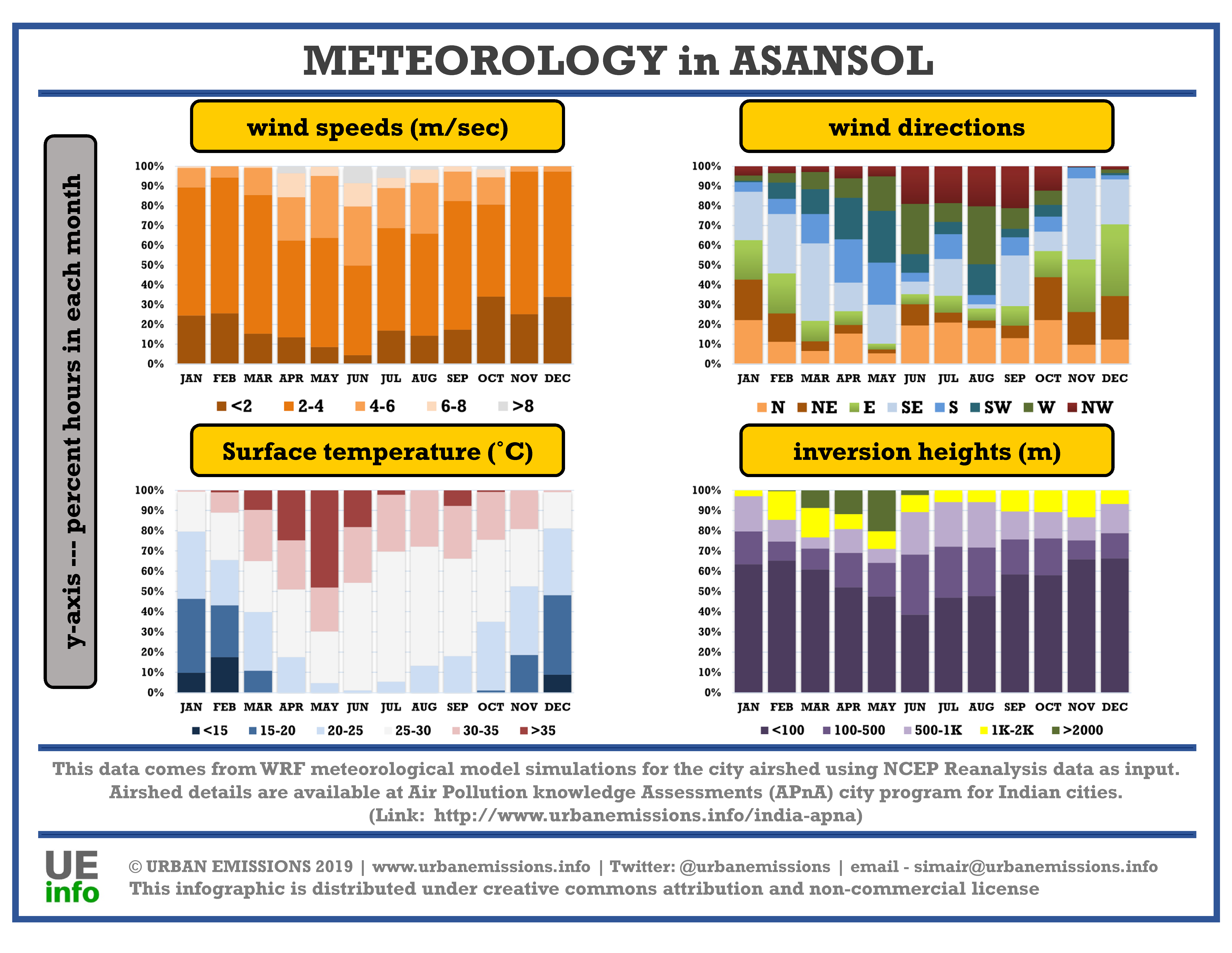
Meteorology fields are important as they have a direct impact on air pollution concentrations. During periods of high precipitation or high speed winds, emissions from a city are swept away and do not have an impact on concentrations. On the other hand, during the winter months when temperatures and inversion heights are low, there is a greater impact of emissions on pollution concentrations. Low temperatures also affect behaviour through the need for space and water heating – which in turn has increases emissions.
We processed the NCEP Reanalysis global meteorological fields from 2010 to 2018 through the 3D-WRF meteorological model. A summary of the data for one year, averaged for the city’s airshed is presented below by month. Download the processed data which includes information on year, month, day, hour, precipitation (mm/hour), mixing height (m), temperature (C), wind speed (m/sec), and wind direction (degrees) – key parameters which determine the intensity of dispersion of emissions.
Multi-Pollutant Emission Inventory
We compiled an emissions inventory for the Asansol region for the following pollutants – sulfur dioxide (SO2), nitrogen oxides (NOx), carbon monoxide (CO), non-methane volatile organic compounds (NMVOCs), carbon dioxide (CO2); and particulate matter (PM) in four bins (a) coarse PM with size fraction between 2.5 and 10 μm (b) fine PM with size fraction less than 2.5 μm (c) black carbon (BC) and (d) organic carbon (OC), for year 2015 and projected to 2030. In Phase 1, base year for all the calculations was 2015. In Phase 2, all the calculations are updated for year 2018.
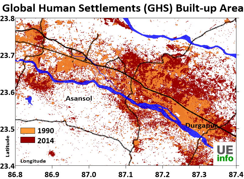 We customized the SIM-air family of tools to fit the base information collated from disparate sources. Apart from the official reports, resource material ranges from GIS databases of land use, land cover, roads and rail lines, water bodies, built up area (represented in the adjacent figure), commercial activities (such as hotels, hospitals, kiosks, restaurants, malls, cinema complexes, traffic intersections, worship points, industrial hubs, and telecom towers), to population density and meteorology at the finest spatial resolution possible (1-km). A detailed description of these resources is published as a journal article in 2019, which also includes a summary of baselines and pollution analysis for 20 Indian cities.
This emissions inventory is based on available local activity and fuel consumption estimates for the selected urban airshed (represented in the grid above). This information is collated from multiple agencies ranging from the central pollution control board, state pollution control board, census bureau, national sample survey office, ministry of road transport and highways, annual survey of industries, central electrical authority, ministry of heavy industries, and municipal waste management, and publications from academic and non-governmental institutions.
For the road transport emissions inventory, besides the total number of vehicles and their usage information, we also utilized vehicle speed information to spatially and temporally allocate the estimated emissions to the respective grids. This is a product of google maps services. For the city of Asansol, we extracted the speed information for representative routes across the city for multiple days. This data is summarized below for a quick look.
 |
Click here for gridded anime |
Railways also is a big contributor to the economy of Asansol. Railways were the first employer in the city and they are credited with developing the city in the late 19th century. Other industries include Dishergarh Power Supply, Damodar Valley Corporation, Hindustan Cables Limited and cement factories. Within the city, the main mode of public transportation consists of a network of cycle rickshaws, auto rickshaws and buses.
 |
 |
 |
 |
 |
 |
The summary for a city’s emissions inventory does not include natural emission sources (like dust storms, lightning, and seasalt) and seasonal open (agricultural and forest) fires. However, these are included in the overall chemical transport modeling in the national scale simulations. These emission sources are accounted in the concentration calculation as an external (also known as boundary or long-range) contribution to the city’s air quality.
Projections to 2030 under the business as usual scenario are influenced by the city’s social, economic, landuse, urban, and industrial layout and hence the projected (increasing and decreasing) rates that we assume are an estimate only. We based the vehicle growth rate on the sales projection numbers; industrial growth on the gross domestic product of the state; domestic sector, construction activities, brick demand, diesel usage in the generator sets, and open waste burning on population growth rates and notes from the municipalities on plans to implement waste management programs. We used these estimates to evaluate the trend in the total emissions and their likely impact on ambient PM2.5 concentrations through 2030.
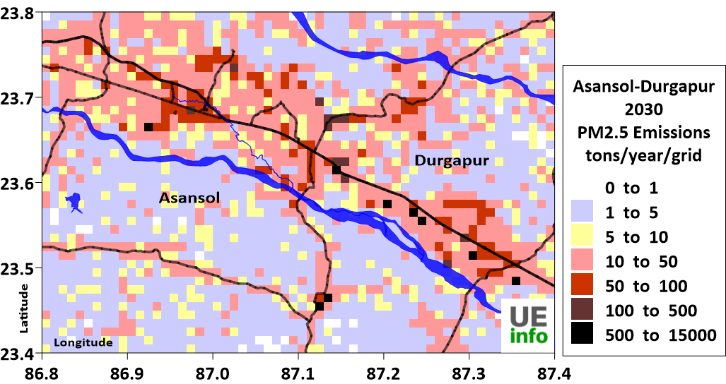
The emissions inventory was then spatially segregated at a 0.01° grid resolution in longitude and latitude (equivalent of 1 km) to create a spatial map of emissions for each pollutant (PM2.5, PM10, SO2, NOx, CO and VOCs). The gridded PM2.5 emissions and the total (shares by sector) emissions are presented below.
Gridded PM2.5 Emissions (2018 and 2030)
 |
 |
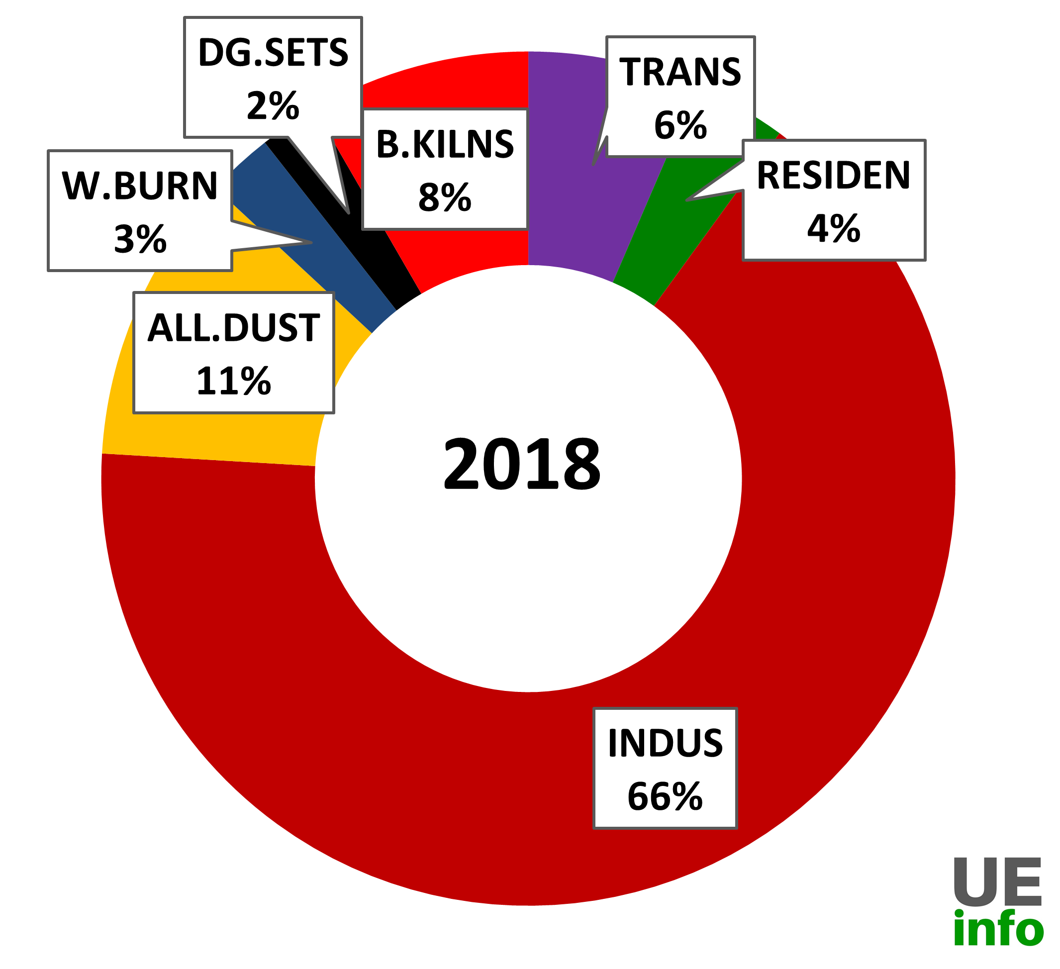
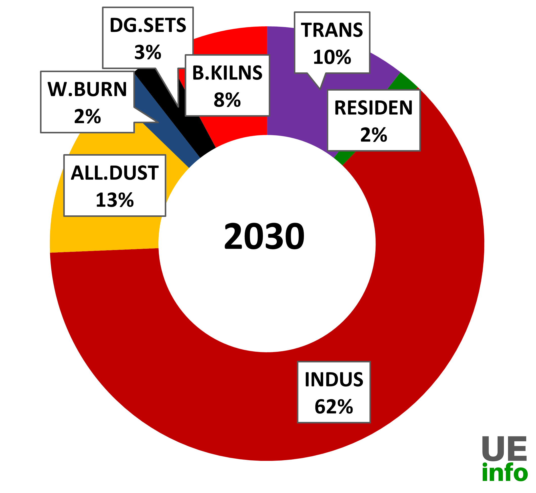
Total PM2.5 Emissions by Sector 2018-2030
 |
 |
 |
TRANS = transport emissions from road, rail, aviation, and shipping (for coastal cities); RESIDEN = residential emissions from cooking, heating, and lighting activities; INDUS = industrial emissions from small, medium, and heavy industries (including power generation); ALL.DUST = dust emissions from road re-suspension and construction activities; W.BURN = open waste burning emissions; DG.SETS = diesel generator set emissions; B.KILNS = brick kiln emissions (not included in the industrial emissions)
Total Estimated Emissions by Sector for 2018 (units – tons/year)
| Asansol | PM2.5 | PM10 | BC | OC | NOx | CO | VOC | SO2 |
|---|---|---|---|---|---|---|---|---|
| Transport emissions from road, rail, aviation, and shipping (for coastal cities) | 4,500 | 4,700 | 1,800 | 1,450 | 18,100 | 177,650 | 30,750 | 200 |
| Residential emissions from cooking, heating, and lighting activities | 2,450 | 2,600 | 550 | 1,150 | 350 | 39,450 | 3,700 | 1,150 |
| Industrial emissions from small, medium, and heavy industries (including power generation) | 45,750 | 51,150 | 5,100 | 4,300 | 121,450 | 77,050 | 249,000 | 6,800 |
| Dust emissions from road re-suspension and construction activities | 7,600 | 46,550 | - | - | - | - | - | - |
| Open waste burning emissions | 1,750 | 1,850 | 150 | 1,050 | 50 | 8,350 | 1,700 | 50 |
| Diesel generator set emissions | 1,550 | 1,650 | 800 | 450 | 10,400 | 33,300 | 15,000 | 250 |
| Brick kiln emissions (not included in the industrial emissions) | 5,800 | 5,850 | 1,400 | 1,800 | 10,000 | 69,900 | 5,800 | 4,250 |
| 69,400 | 114,350 | 9,800 | 10,200 | 160,350 | 405,700 | 305,950 | 12,700 |
Chemical Transport Modeling
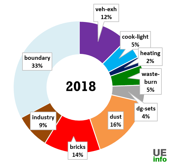
We calculated the ambient PM2.5 concentrations and the source contributions, using gridded emissions inventory, 3D meteorological data (from WRF), and the CAMx regional chemical transport model. The model simulates concentrations at 0.01° grid resolution and sector contributions for the urban area, which include contributions from primary emissions, secondary sources via chemical reactions, and long range transport via boundary conditions (represented as “boundary” in the pie graph below).
 |
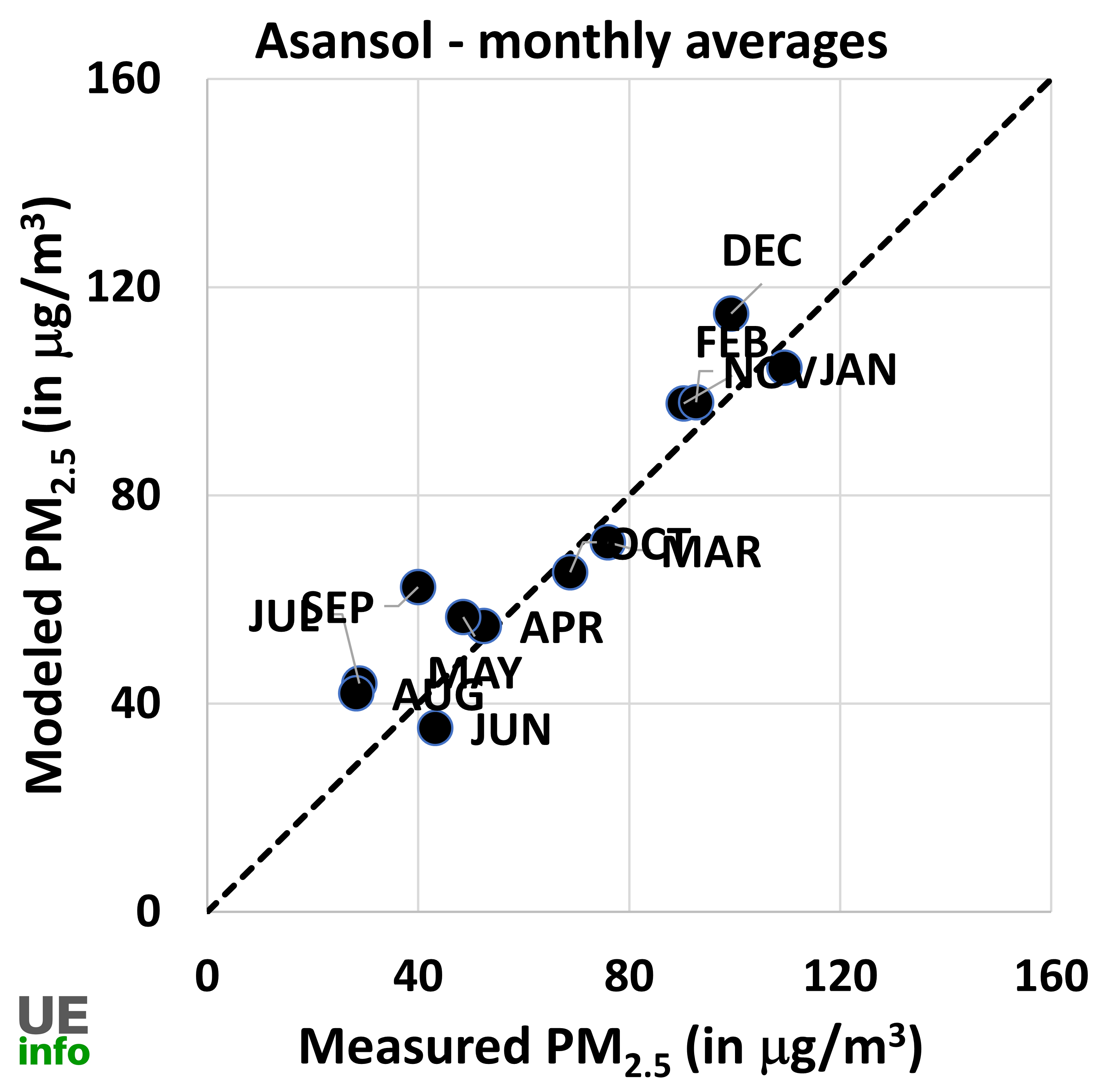 |
The ribbon graph shows the variation for average PM2.5 pollution by month. Due to precipitation during the monsoon, usually pollution levels dip and may fall within national air pollution standards, however most cities are unable to attain these standards at other times of the year. We consolidated all the PM2.5 data from the continuous monitoring stations operating within the modeling domain, for the period of 2018-19 and compared against the model results. The scatter plot presents a comparison of 24-hr average PM2.5 concentrations by month. Modeled data is for the urban parts of the city.
The following is a map of annual average PM2.5 pollution for the city of Asansol. The main sources contributing towards PM2.5 in 2018 are in the pie-chart on the left. The change in contributions in 2030 from different sources are shown on the right.
 |
 |
 |
There is a temporal variation in source contributions and spatial contributions depending on meteorological factors. We have a map of monthly average PM2.5 levels as well as their source contributions for every month in the charts below.
 |
 |
Satellite Data Derived Surface PM2.5 Concentrations
The results of satellite data derived concentrations are useful for evaluating annual trends in pollution levels and are not a proxy for on-ground monitoring networks. This data is estimated using satellite feeds and global chemical transport models. Satellites are not measuring one location all the time, instead, a combination of satellites provide a cache of measurements that are interpreted using global chemical transport models (GEOS-Chem) to represent the vertical mix of pollution and estimate ground-based concentrations with the help of previous ground-based measurements. The global transport models rely on gridded emission estimates for multiple sectors to establish a relationship with satellite observations over multiple years. These databases were also used to study the global burden of disease, which estimated air pollution as the top 10 causes of premature mortality and morbidity in India. A summary of PM2.5 concentrations for the period of 1998 to 2016 for the city of Asansol is presented below. The global PM2.5 files are available for download and further analysis @ Dalhousie University.
The graphs for other district PM2.5 concentrations for this period, maps of national averages, and year-wise changes are available here. The data for district level PM2.5 concentrations for 1998-2016 period for can downloaded here.
Monitoring
We present below a summary of the ambient monitoring data available under the National Ambient Monitoring Program (NAMP), operated and maintained by the Central Pollution Control Board (CPCB, New Delhi, India). In Asansol, as of November 2018, there are 0 continuous and 2 manual air quality stations in operation. An archive of all the data from the NAMP network from stations across India for the period of 2011-2015 is available here.
 |
 |
 |
Resource Material
- CPCB repository of continuous air monitoring data (Link)
- Regional Offices, West Bengal Pollution Control Board (Link)
- Website of Atal Mission for Rejuvenation and Urban Transformation, Asansol Municipal Corporation (Link)
- “Approved Green City Mission Plan”, Urban Development and Municipal Affairs Department, Government of West Bengal. (2017). Pages 7, 15-16 (Link)
- “Land Use Development Control Plan 2025 for Asansol Sub-Division”, Asansol Durgapur Development Authority. (2015) (Link)
- “Implementation of Action Plan for Critically Polluted Area (Asansol)”, West Bengal Pollution Control Board. (2014) (Link)
- “Operations in Raniganj (South)”, Great Eastern Energy Corporation Limited (Link)
- “Ambient air quality status in Raniganj-Asansol area, India”, Reddy, GS and Ruj, B. (2003) (Journal Article Link)
- “Biomonitoring of air quality in the industrial town of asansol using the air pollution tolerance index approach”, Choudhury, P. and Banerjee, D. (2009) (Journal Article Link)
- “Characterization of different road dusts in opencast coal mining areas of India”, Mandal, K. et. al. (2011) (Journal Article Link)
- “Fugitive Methane Emissions from Indian Coal Mining and Handling Activities: Estimates, Mitigation and Opportunities for its Utilization to Generate Clean Energy”, Singh, A.K. and Kumar, J. (2016) (Journal Article Link)
Back to the APnA page.
All the analysis and results are sole responsibility of the authors @ UrbanEmissions.Info. Please send you comments and questions to simair@urbanemissions.info