Puducherry (formerly Pondicherry) is a union territory on the east coast of India, 150 km from Chennai and is bordered by the state of Tamil Nadu. Pondicherry was a former French territory and secured its independent status only in 1954. The city is synonymous with Auroville – which is a community and township founded by the Aurobindo Ashram.
Fisheries, agriculture and tourism are its biggest sectors, followed by light manufacturing, textiles, leather and electronics. A distinctive feature of the region is the quality of road network. Puducherry district has a road length of 2,552 km the highest density in the country. The population of Pondicherry as per the 2011 census was a quarter of a million.
![]() The city itself is tiny – only 20 sq.km. We have extended the airshed to include the port city of Cuddalore to the South of Pondicherry. Apart from fishing and port related industries, Cuddalore hosts chemical industries in the SIPCOT industrial estate. To assess Puducherry’s air quality, we selected an airshed covering 40km x 40km. This domain is further segregated into 1km grids, to study the spatial variations in the emission and the pollution loads.
The city itself is tiny – only 20 sq.km. We have extended the airshed to include the port city of Cuddalore to the South of Pondicherry. Apart from fishing and port related industries, Cuddalore hosts chemical industries in the SIPCOT industrial estate. To assess Puducherry’s air quality, we selected an airshed covering 40km x 40km. This domain is further segregated into 1km grids, to study the spatial variations in the emission and the pollution loads.
Meteorology fields are important as they have a direct impact on air pollution concentrations. During periods of high precipitation or high speed winds, emissions from a city are swept away and do not have an impact on concentrations. On the other hand, during the winter months when temperatures and inversion heights are low, there is a greater impact of emissions on pollution concentrations. Low temperatures also affect behaviour through the need for space and water heating – which in turn has increases emissions.
We processed the NCEP Reanalysis global meteorological fields from 2010 to 2018 through the 3D-WRF meteorological model. A summary of the data for one year, averaged for the city’s airshed is presented below by month. Download the processed data which includes information on year, month, day, hour, precipitation (mm/hour), mixing height (m), temperature (C), wind speed (m/sec), and wind direction (degrees) – key parameters which determine the intensity of dispersion of emissions.

Multi-Pollutant Emission Inventory
We compiled an emissions inventory for the Puducherry region for the following pollutants – sulfur dioxide (SO2), nitrogen oxides (NOx), carbon monoxide (CO), non-methane volatile organic compounds (NMVOCs), carbon dioxide (CO2); and particulate matter (PM) in four bins (a) coarse PM with size fraction between 2.5 and 10 μm (b) fine PM with size fraction less than 2.5 μm (c) black carbon (BC) and (d) organic carbon (OC), for year 2015 and projected to 2030. In Phase 1, base year for all the calculations was 2015. In Phase 2, all the calculations are updated for year 2018.
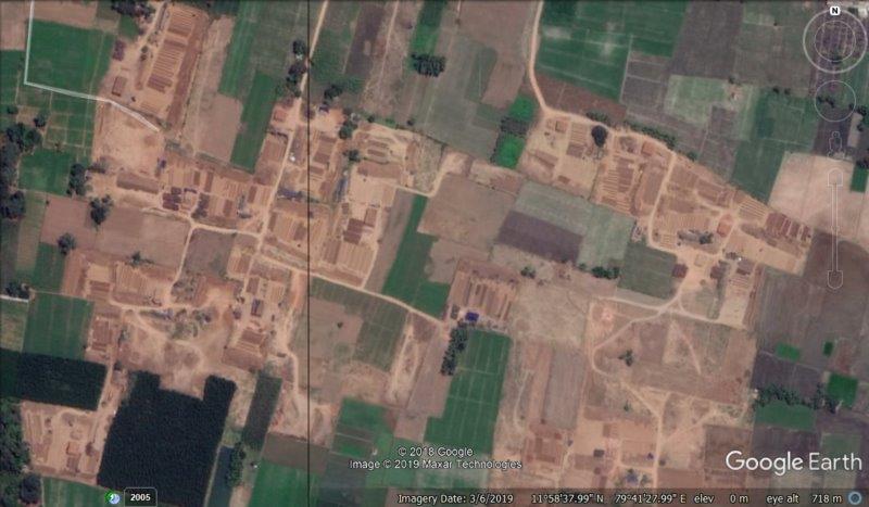
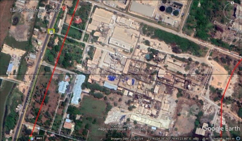
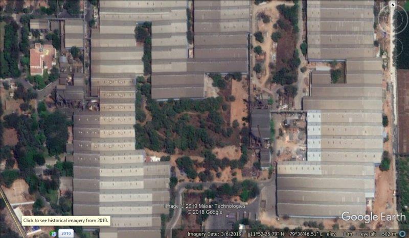
 We customized the SIM-air family of tools to fit the base information collated from disparate sources. Apart from the official reports, resource material ranges from GIS databases of land use, land cover, roads and rail lines, water bodies, built up area (represented in the adjacent figure), commercial activities (such as hotels, hospitals, kiosks, restaurants, malls, cinema complexes, traffic intersections, worship points, industrial hubs, and telecom towers), to population density and meteorology at the finest spatial resolution possible (1-km). A detailed description of these resources is published as a journal article in 2019, which also includes a summary of baselines and pollution analysis for 20 Indian cities.
This emissions inventory is based on available local activity and fuel consumption estimates for the selected urban airshed (represented in the grid above). This information is collated from multiple agencies ranging from the central pollution control board, state pollution control board, census bureau, national sample survey office, ministry of road transport and highways, annual survey of industries, central electrical authority, ministry of heavy industries, and municipal waste management, and publications from academic and non-governmental institutions.
For the road transport emissions inventory, besides the total number of vehicles and their usage information, we also utilized vehicle speed information to spatially and temporally allocate the estimated emissions to the respective grids. This is a product of google maps services. For the city of Puducherry, we extracted the speed information for representative routes across the city for multiple days. This data is summarized below for a quick look.
 |
 |
 |
 |
 |
 |
 |
 |
 |
 |
 |
The summary for a city’s emissions inventory does not include natural emission sources (like dust storms, lightning, and seasalt) and seasonal open (agricultural and forest) fires. However, these are included in the overall chemical transport modeling in the national scale simulations. These emission sources are accounted in the concentration calculation as an external (also known as boundary or long-range) contribution to the city’s air quality.
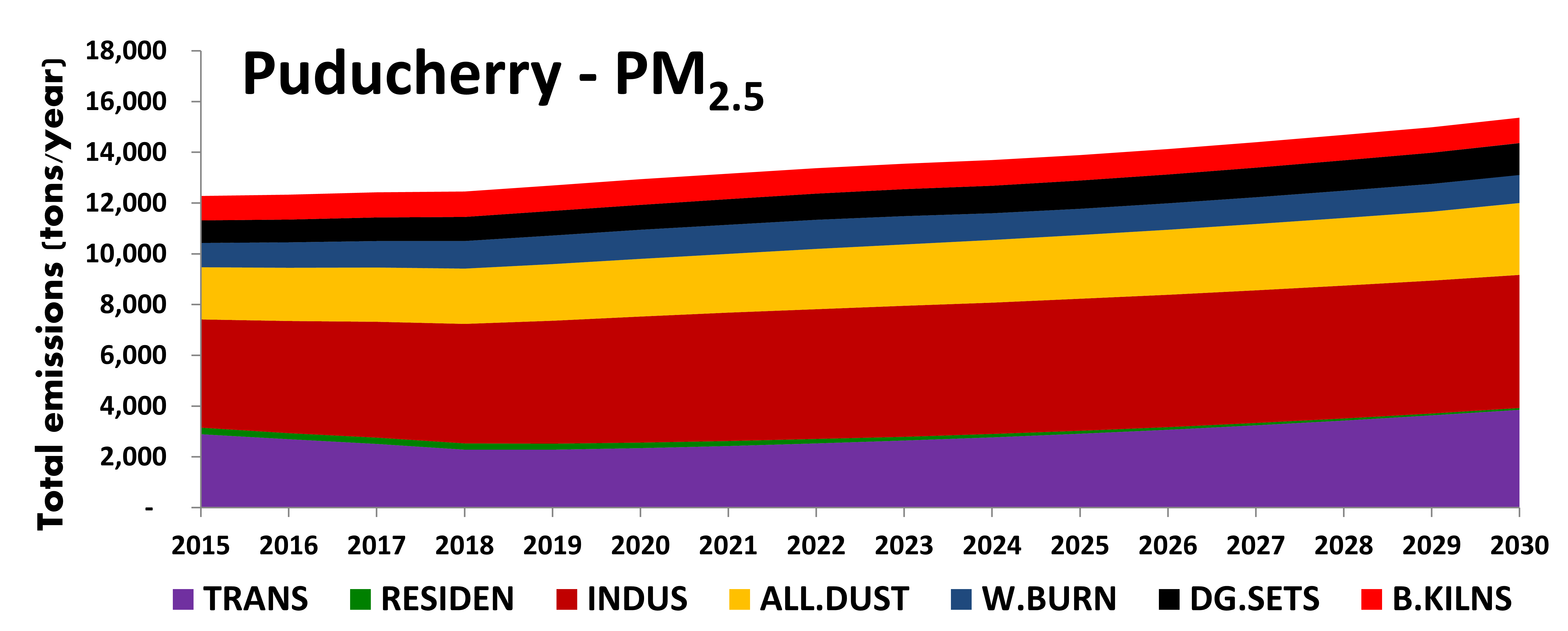
Projections to 2030 under the business as usual scenario are influenced by the city’s social, economic, landuse, urban, and industrial layout and hence the projected (increasing and decreasing) rates that we assume are an estimate only. We based the vehicle growth rate on the sales projection numbers; industrial growth on the gross domestic product of the state; domestic sector, construction activities, brick demand, diesel usage in the generator sets, and open waste burning on population growth rates and notes from the municipalities on plans to implement waste management programs. We used these estimates to evaluate the trend in the total emissions and their likely impact on ambient PM2.5 concentrations through 2030.
The emissions inventory was then spatially segregated at a 0.01° grid resolution in longitude and latitude (equivalent of 1 km) to create a spatial map of emissions for each pollutant (PM2.5, PM10, SO2, NOx, CO and VOCs). The gridded PM2.5 emissions and the total (shares by sector) emissions are presented below.
Gridded PM2.5 Emissions (2018 and 2030)
 |
 |
Total PM2.5 Emissions by Sector 2018-2030
 |
 |
 |
TRANS = transport emissions from road, rail, aviation, and shipping (for coastal cities); RESIDEN = residential emissions from cooking, heating, and lighting activities; INDUS = industrial emissions from small, medium, and heavy industries (including power generation); ALL.DUST = dust emissions from road re-suspension and construction activities; W.BURN = open waste burning emissions; DG.SETS = diesel generator set emissions; B.KILNS = brick kiln emissions (not included in the industrial emissions)
Total Estimated Emissions by Sector for 2018 (units – tons/year)
| Puducherry | PM2.5 | PM10 | BC | OC | NOx | CO | VOC | SO2 |
|---|---|---|---|---|---|---|---|---|
| Transport emissions from road, rail, aviation, and shipping (for coastal cities) | 2,300 | 2,400 | 700 | 800 | 10,400 | 104,450 | 34,350 | 100 |
| Residential emissions from cooking, heating, and lighting activities | 250 | 250 | 50 | 150 | 50 | 3,800 | 400 | 50 |
| Industrial emissions from small, medium, and heavy industries (including power generation) | 4,700 | 4,750 | 1,750 | 950 | 1,750 | 4,850 | 500 | 1,150 |
| Dust emissions from road re-suspension and construction activities | 2,200 | 13,250 | - | - | - | - | - | - |
| Open waste burning emissions | 1,100 | 1,150 | 100 | 650 | 50 | 5,200 | 1,050 | 50 |
| Diesel generator set emissions | 950 | 1,000 | 450 | 300 | 6,350 | 20,300 | 9,150 | 150 |
| Brick kiln emissions (not included in the industrial emissions) | 1,000 | 1,000 | 250 | 300 | 1,700 | 11,150 | 1,100 | 600 |
| 12,500 | 23,800 | 3,300 | 3,150 | 20,300 | 149,750 | 46,550 | 2,100 |
Chemical Transport Modeling
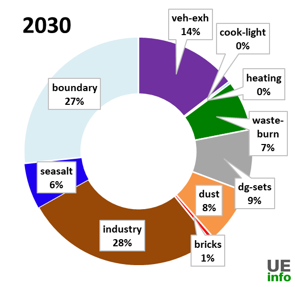
We calculated the ambient PM2.5 concentrations and the source contributions, using gridded emissions inventory, 3D meteorological data (from WRF), and the CAMx regional chemical transport model. The model simulates concentrations at 0.01° grid resolution and sector contributions for the urban area, which include contributions from primary emissions, secondary sources via chemical reactions, and long range transport via boundary conditions (represented as “boundary” in the pie graph below).

The ribbon graph shows the variation for average PM2.5 pollution by month. Due to precipitation during the monsoon, usually pollution levels dip and may fall within national air pollution standards, however most cities are unable to attain these standards at other times of the year.
The following is a map of annual average PM2.5 pollution for the city of Puducherry. The main sources contributing towards PM2.5 in 2018 are in the pie-chart on the left. The change in contributions in 2030 from different sources are shown on the right.
 |
 |
 |
There is a temporal variation in source contributions and spatial contributions depending on meteorological factors. We have a map of monthly average PM2.5 levels as well as their source contributions for every month in the charts below.
 |
 |
Satellite Data Derived Surface PM2.5 Concentrations
The results of satellite data derived concentrations are useful for evaluating annual trends in pollution levels and are not a proxy for on-ground monitoring networks. This data is estimated using satellite feeds and global chemical transport models. Satellites are not measuring one location all the time, instead, a combination of satellites provide a cache of measurements that are interpreted using global chemical transport models (GEOS-Chem) to represent the vertical mix of pollution and estimate ground-based concentrations with the help of previous ground-based measurements. The global transport models rely on gridded emission estimates for multiple sectors to establish a relationship with satellite observations over multiple years. These databases were also used to study the global burden of disease, which estimated air pollution as the top 10 causes of premature mortality and morbidity in India. A summary of PM2.5 concentrations for the period of 1998 to 2016 for the city of Puducherry is presented below. The global PM2.5 files are available for download and further analysis @ Dalhousie University.
The graphs for other district PM2.5 concentrations for this period, maps of national averages, and year-wise changes are available here. The data for district level PM2.5 concentrations for 1998-2016 period for can downloaded here.
Monitoring
We present below a summary of the ambient monitoring data available under the National Ambient Monitoring Program (NAMP), operated and maintained by the Central Pollution Control Board (CPCB, New Delhi, India). In Puducherry, as of November 2018, there are 0 continuous and 2 manual air quality stations in operation. An archive of all the data from the NAMP network from stations across India for the period of 2011-2015 is available here.
 |
 |
 |
Resource Material
-
- CPCB repository of continuous air monitoring data (Link)
Back to the APnA page.
All the analysis and results are sole responsibility of the authors @ UrbanEmissions.Info. Please send you comments and questions to simair@urbanemissions.info